RF - Antenna Basics

This article provides an introduction to the principles and fundamental parameters of antennas.

Antenna Principles

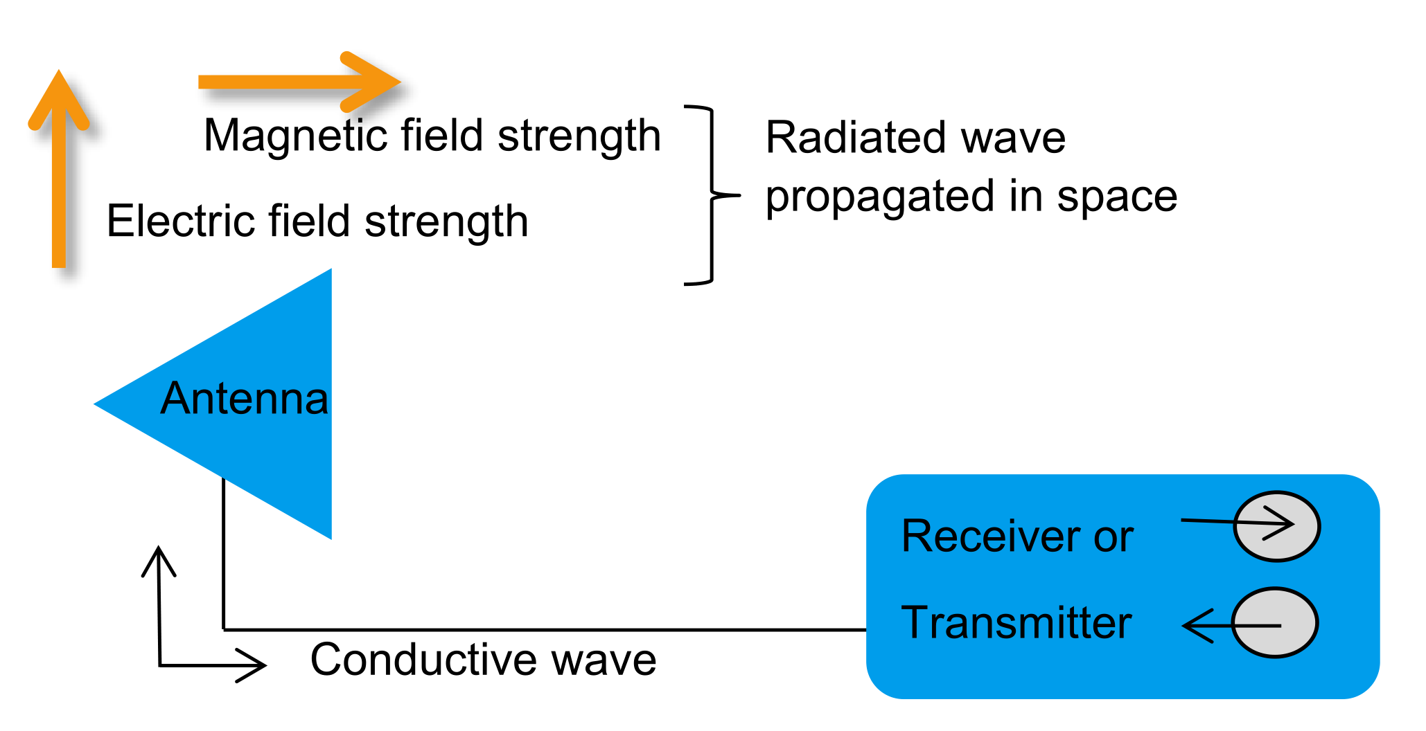
An antenna is a transducer that converts electrical signals on a conductor into electromagnetic waves in space, or it can collect electromagnetic waves in space and convert them into electrical signals (both modes are theoretically equivalent, except for active antennas).

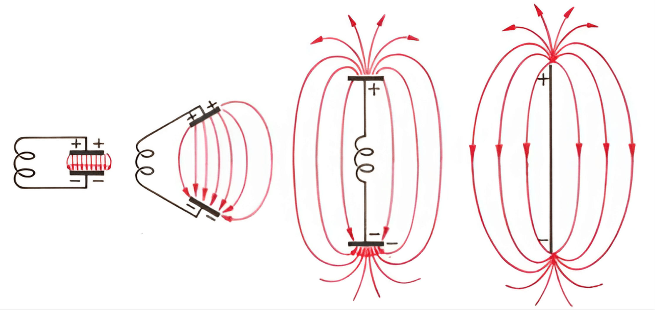
Antennas originated from resonators composed of inductance and parallel-plate capacitors. By separating the parallel plates, the inductance decreases. By separating them a certain distance and considering the inductance of the conductor itself as resonant inductance, a dipole antenna can be formed.

Antenna Parameters

Radiation Density

Assuming an ideal isotropic microwave transmitter, which is a point in space generating spherical waves radiating uniformly in all directions.

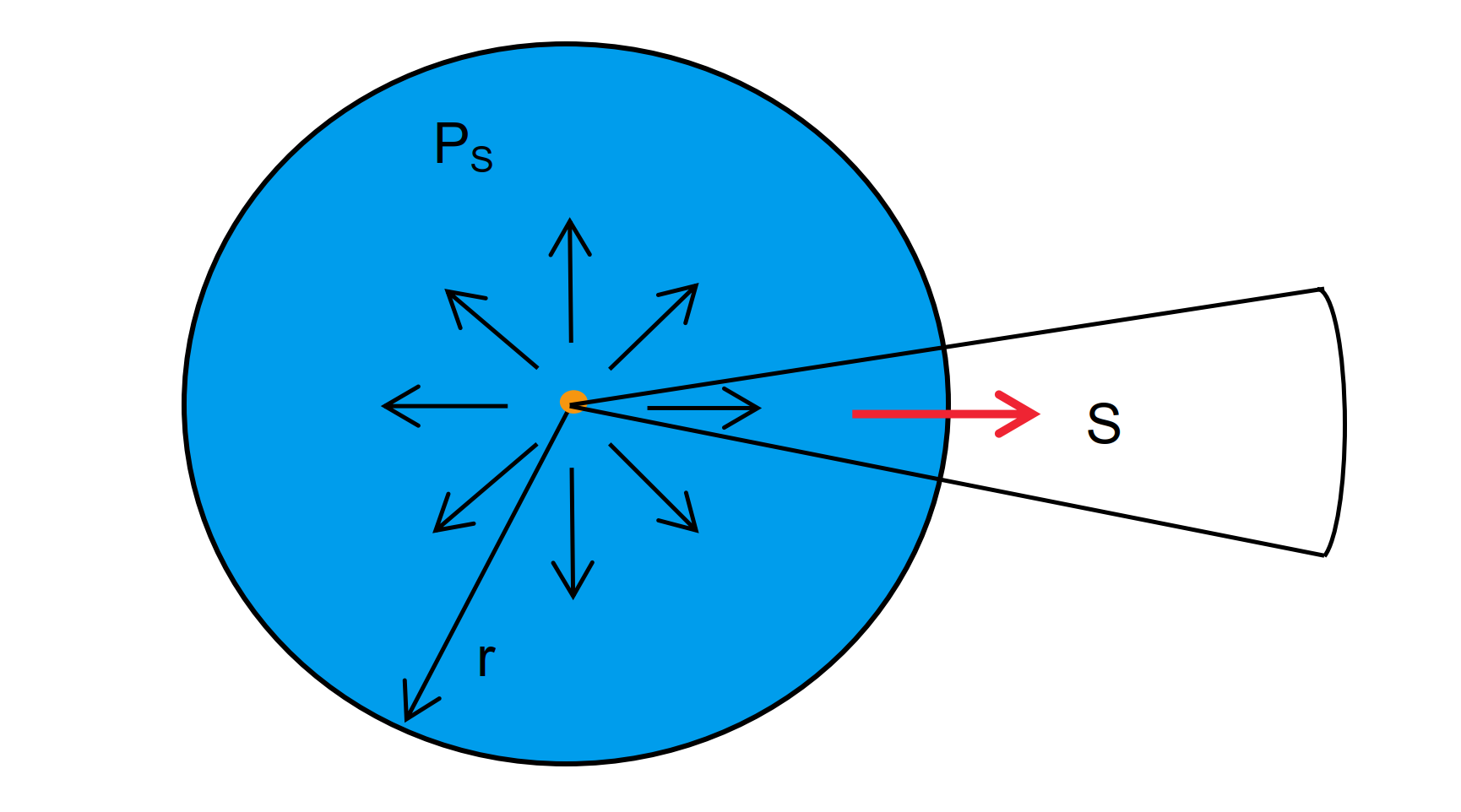
When a transmission power \(P_S\) is applied to this microwave transmitter, the radiation density (also known as power density) at a distance \(r\) is given by:

\[ S = \frac{P_S}{4\pi r^2} \]

Radiation density can also be defined as the product of the electric field and magnetic field strength in the far field:

\[ S = E \cdot H \]

Radiation Pattern

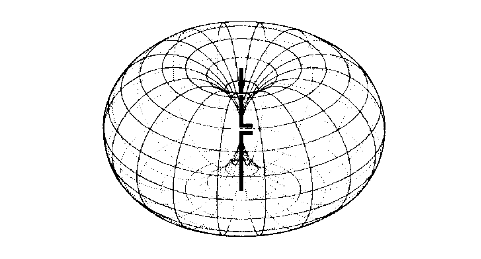
The radiation pattern is used to describe the three-dimensional radiation effects in the far field of an antenna. For an isotropic radiator (referred to as a point source antenna), the radiation is the same in all directions, but it cannot be polarized in a specific direction. For general antennas, such as dipole and monopole antennas, they have directionality. For example, the 3D radiation pattern in free space for a short dipole antenna is shown below. It can be observed that there is no radiation density in the direction of the antenna axis:

In addition to using 3D plots to represent radiation, horizontal and vertical 2D profile plots (also called main plane pattern) are often used. The following images show the horizontal and vertical patterns of a dipole antenna:

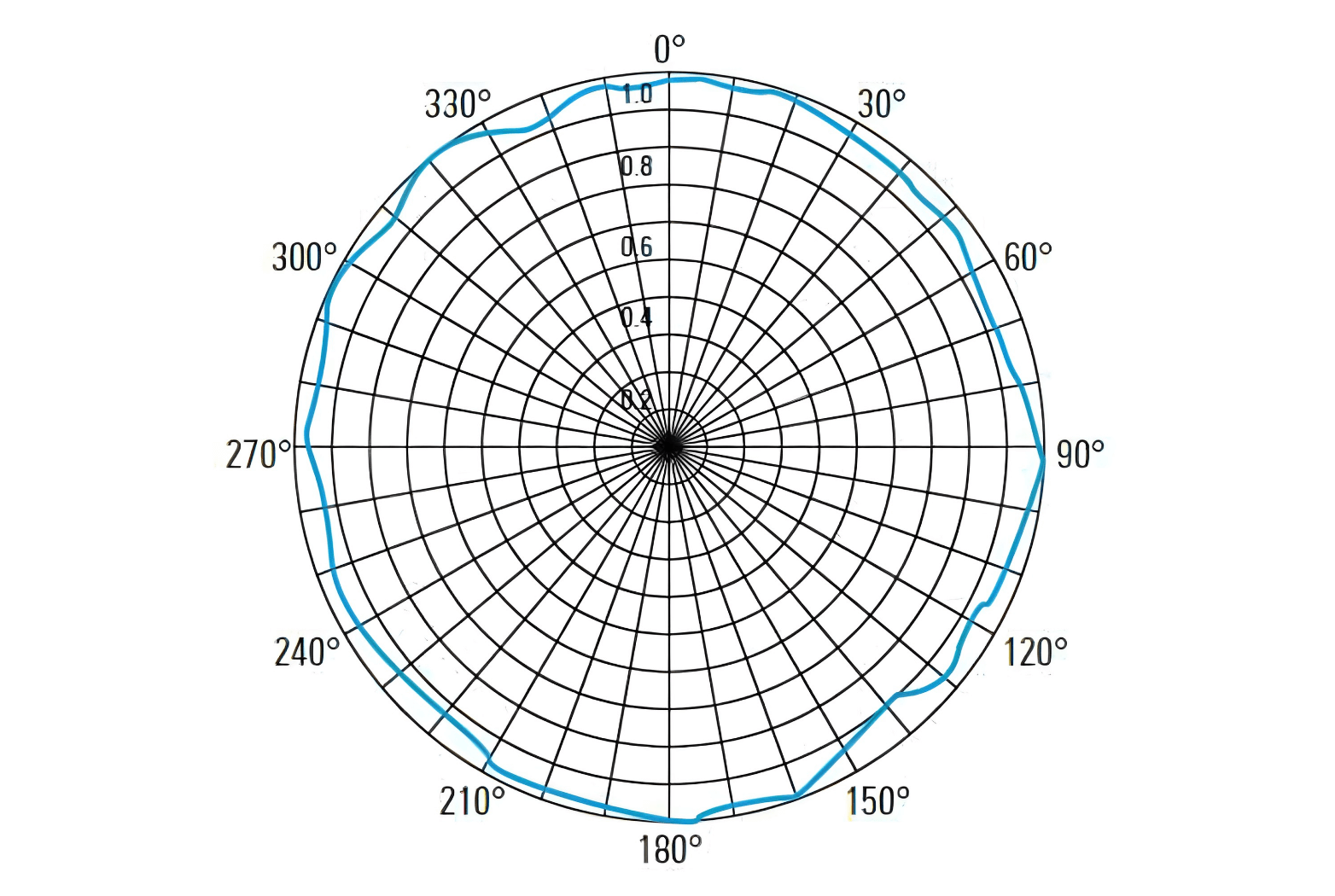
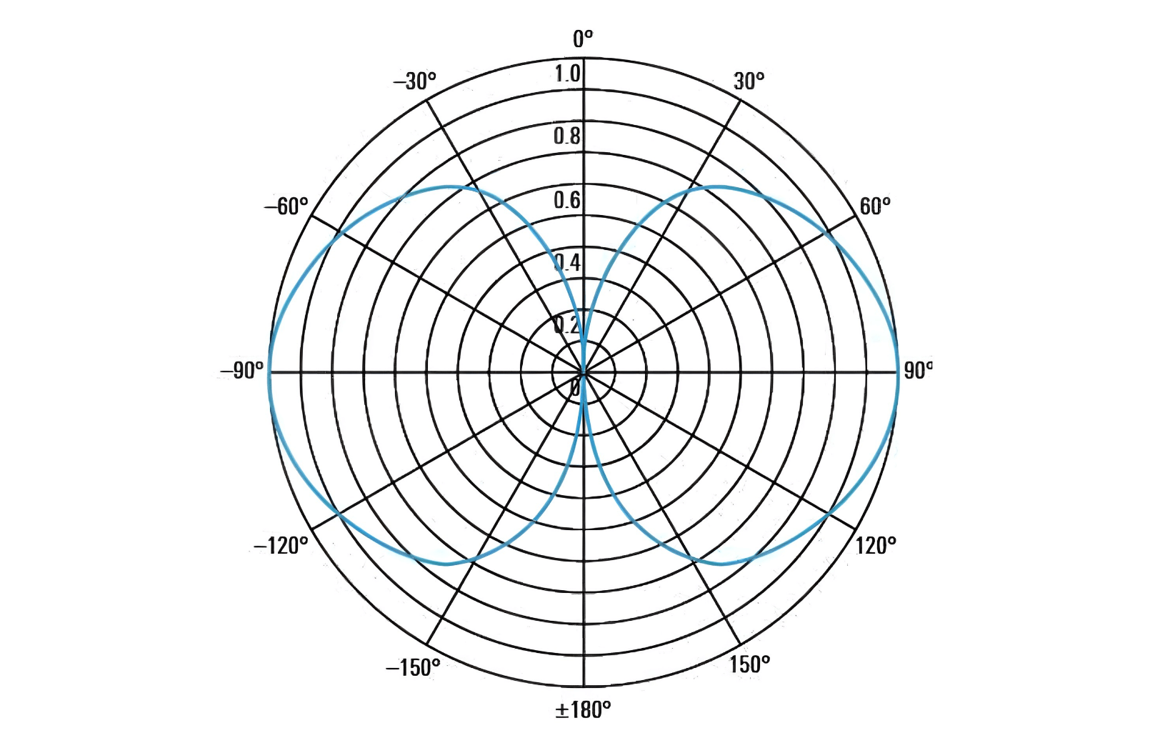
Radiation patterns are typically plotted in polar coordinates, which provide an intuitive understanding of the radiation in each direction. In some cases, such as highly directional antennas, radiation patterns can be represented in Cartesian coordinates (X-Y plane) to highlight details of the main beam and adjacent side lobes more clearly:

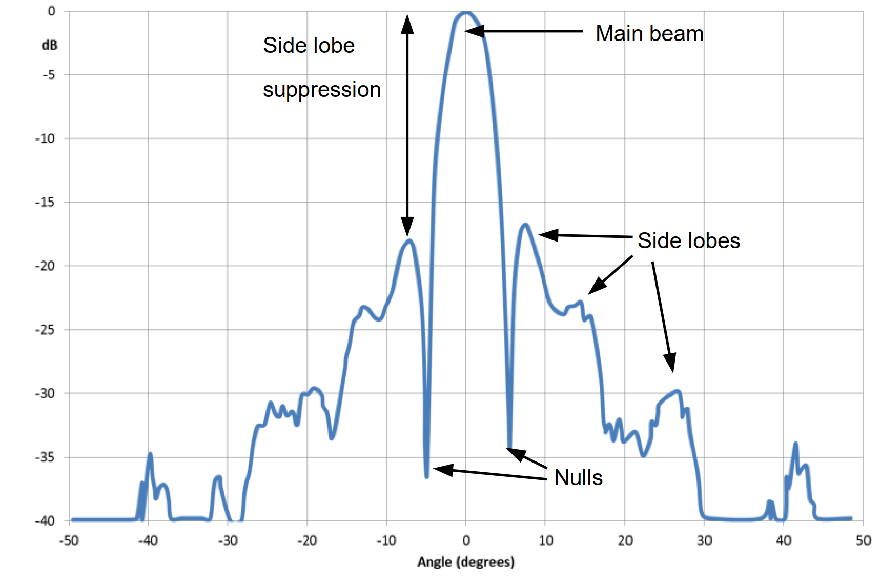
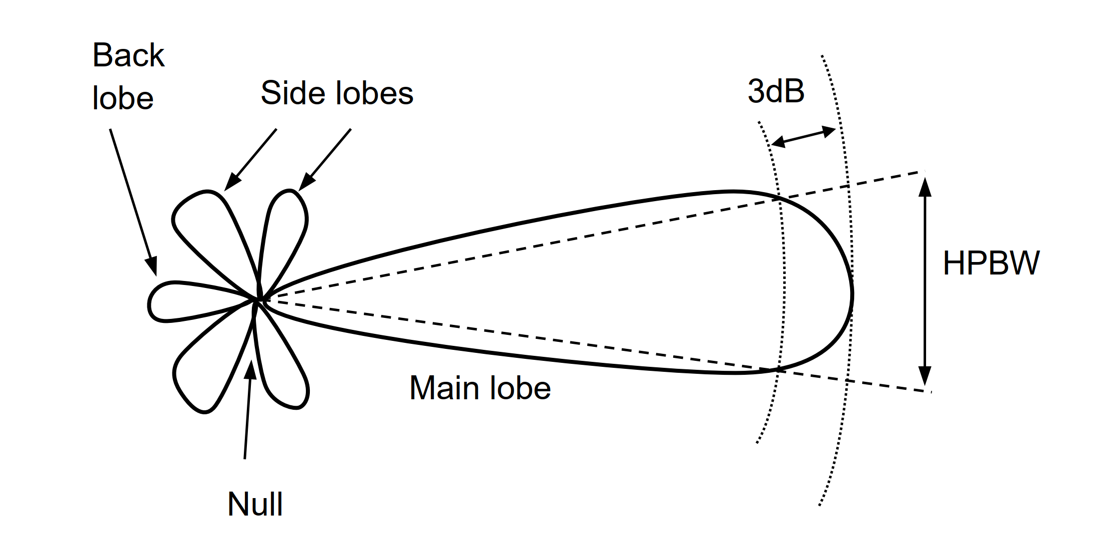
Based on the radiation pattern, various antenna parameters can be observed:

• Side Lobe Suppression (or Side Lobe Level): Indicates the difference between the main lobe and the highest side lobe.
• Half-Power Beamwidth (HPBW): Represents the range between the two angles where the main lobe drops 3dB from its maximum height, typically presented in horizontal and vertical 2D radiation patterns.
• Front-to-Back Ratio: Represents the ratio of the peak gain of a directional antenna in the forward direction to the gain in the back (180°) direction, typically expressed in dB.

Directivity

The antenna's directivity factor \(D\) (also known as the directive gain) represents the ratio of its radiation intensity \(F_{max}\) in the main direction to the radiation intensity \(F_i\) of a lossless point source antenna with the same power (\(P_t\)). Here, we use the Poynting vector to represent power density:

\[ \vec S = \vec E \times \vec H \]

Note: In the far field, \(\vec S\) is perpendicular to \(\vec E\), and both \(\vec S\) and \(\vec E\) are perpendicular to \(\vec H\).

Power density is measured at a distance \(r\) from the antenna. Therefore, when \(F_i = \frac{P_t}{4\pi}\), we can derive:

\[ D = \frac{F_{max}}{F_i} \]

Efficiency

Antenna efficiency \(\eta\) is generally defined as the ratio of the radiated power of an antenna to its input power. High-efficiency antennas radiate most of the input energy, while low-efficiency antennas absorb most of it as losses inside the antenna or reflect it due to impedance mismatch. For passive antennas, whether used for transmitting or receiving, their efficiency is the same, a property known as antenna reciprocity. The formula for antenna radiation efficiency \(\varepsilon_R\) is as follows:

\[ \varepsilon_R = \frac{P_{refl}}{P_{forw}} \cdot 100\% \]

Antenna efficiency is not only expressed as a percentage but is also commonly represented in dB. For example, 10% efficiency is equivalent to -10 dB, and 50% efficiency is equivalent to -3 dB.

The above formula represents the radiation efficiency of the antenna. There is another efficiency called the total efficiency of the antenna, denoted as \(\varepsilon_r\). The relationship between them is that the total efficiency is equal to the radiation efficiency multiplied by the impedance mismatch loss \(M_L\):

\[ \varepsilon_r = M_L \cdot \varepsilon_R \]

Since impedance mismatch loss is between 0 and 1, the total efficiency of the antenna is always less than the radiation efficiency. If the impedance is perfectly matched, the two efficiencies are equal. In practice, antenna efficiency typically refers to the total efficiency considering impedance mismatch loss, so better impedance matching can improve the actual efficiency of the antenna.

Gain

Antenna gain measures the ability of an antenna to transmit or receive signals in a specific direction. Gain is closely related to the antenna's radiation pattern, where a narrower main lobe and smaller side lobes result in higher gain.

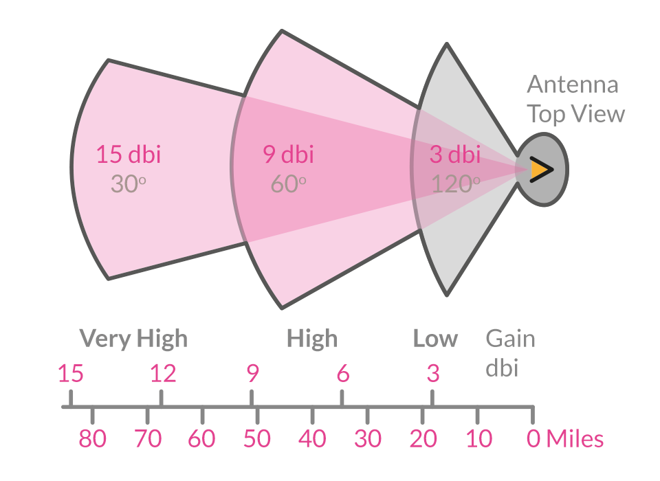
Under the same conditions, higher gain concentrates energy more, narrows the radiation pattern, and allows radio waves to be transmitted over longer distances. However, the coverage angle becomes smaller. Therefore, it is important to choose the antenna gain appropriately in practical applications.

Antenna gain corresponds to the directional coefficient and represents the radiation intensity \(F_{max}\) in the main radiation direction compared to the radiation intensity \(F_{i0}\) produced by a lossless point source antenna with the same power (\(P_{t0}\)). When \(F_{i0} = \frac{P_t}{4\pi}\), we have:

\[ G = \frac{F_{max}}{F_{i0}} \]

Unlike the directional coefficient, gain also takes antenna efficiency \(\eta\) into account:

\[ G = \eta \cdot D \]

If the antenna efficiency is 100%, the gain is equal to the directional coefficient. In reality, efficiency cannot reach 100%, so in practical measurements, gain is more commonly used than the directional coefficient.

Gain and directional coefficient are usually expressed in dB. Gain \(g(dB) = 10 \log G\) and directional coefficient \(d(dB) = 10 \log D\). This leads to the derivation of dBd (relative to a half-wave dipole antenna) and dBi (relative to a point source antenna), where dBi = dBd + 2.15.

Some additional notes about gain:

• Antennas are passive devices and do not generate energy. Antenna gain is a measure of the ability to efficiently concentrate energy in a specific direction for transmitting or receiving electromagnetic waves.
• Antenna gain is produced by the superposition of elements, and higher gain requires a longer antenna length. For every 3 dB increase in gain, the volume doubles.

Practical Gain

The definition of gain assumes perfect impedance matching between the antenna and the source, which is rarely achievable in practice. Therefore, the gain value measured under actual, non-ideal matching conditions is known as the antenna's practical gain. Its formula is defined as follows:

\[ G_{pract} = (1 - |r|^2) \cdot G \]

Here, \(r\) represents the reflection coefficient, which will be explained in detail below.

Effective Area

The effective area of an antenna, denoted as \(A_W\), is a parameter specifically defined for receiving antennas. It measures the antenna's ability to pick up signals and is defined as the ratio of the maximum received power \(P_{rmax}\) to the plane wave power density \(S\):

\[ A_W = \frac{P_{rmax}}{S} \]

For aperture antennas like parabolic reflectors or planar arrays, the effective area is the physical area multiplied by the aperture efficiency \(q\).

\[ A_W = A_g \cdot q \]

The effective area of the antenna is also related to its gain (and vice versa):

\[ A_W = \frac{\lambda^2}{4\pi} \cdot G \]

Input Impedance

The input impedance of an antenna is a critical parameter, and it is a complex value composed of a real resistance and an imaginary reactance:

\[ Z_{in} = R_{in} + jX_{in} \]

The real resistance, \(R_{in\), is composed of the radiation resistance \(R_R\) and the loss resistance \(R_L\):

\[ R_{in} = R_R + R_L \]

For small antennas, calculating the radiation resistance \(R_R\) requires specifying its position on the antenna because it is space-dependent (the ratio of radiated power to the root mean square current). The same applies to the antenna current; you need to specify the antenna feed point to determine the maximum current value.

If the antenna operates at a resonant state, the imaginary part of the input impedance is zero. Electrically short linear antennas typically exhibit capacitance (\(X_{in} < 0\)), while electrically long linear antennas typically exhibit inductance (\(X_{in} > 0\)).

Nominal Impedance

The nominal impedance, \(Z_n\), is usually defined as the characteristic impedance of the antenna feedline, often 50Ω. Typically, the antenna impedance should match this value.

Impedance Matching

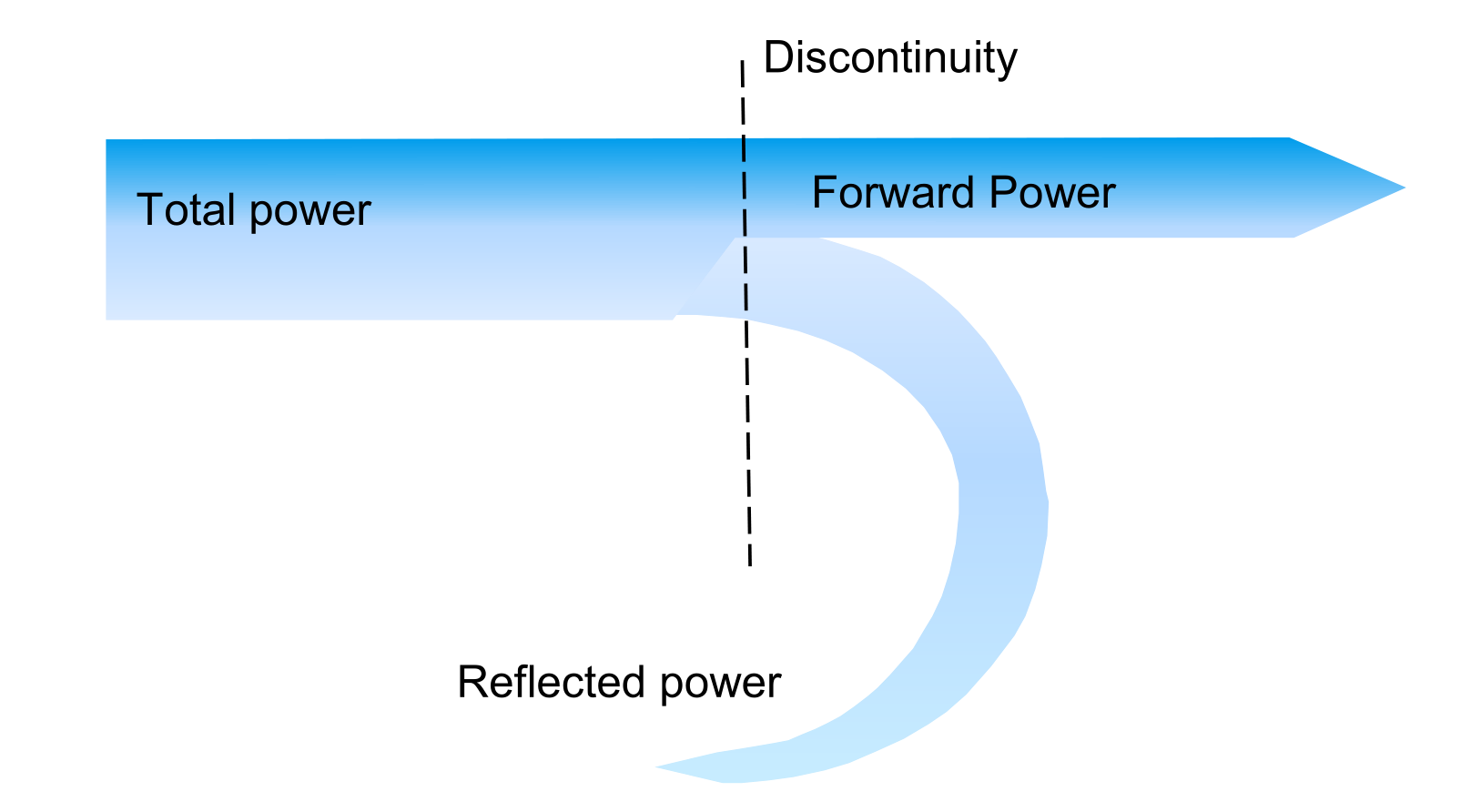
Mismatched impedances between the antenna, feedline, and the source end can lead to discontinuities. In the example below, when energy is transmitted from the source end, some of it is reflected back and cannot reach the antenna, affecting transmission efficiency. Conversely, not all the energy received by the antenna can be transmitted to the receiver:

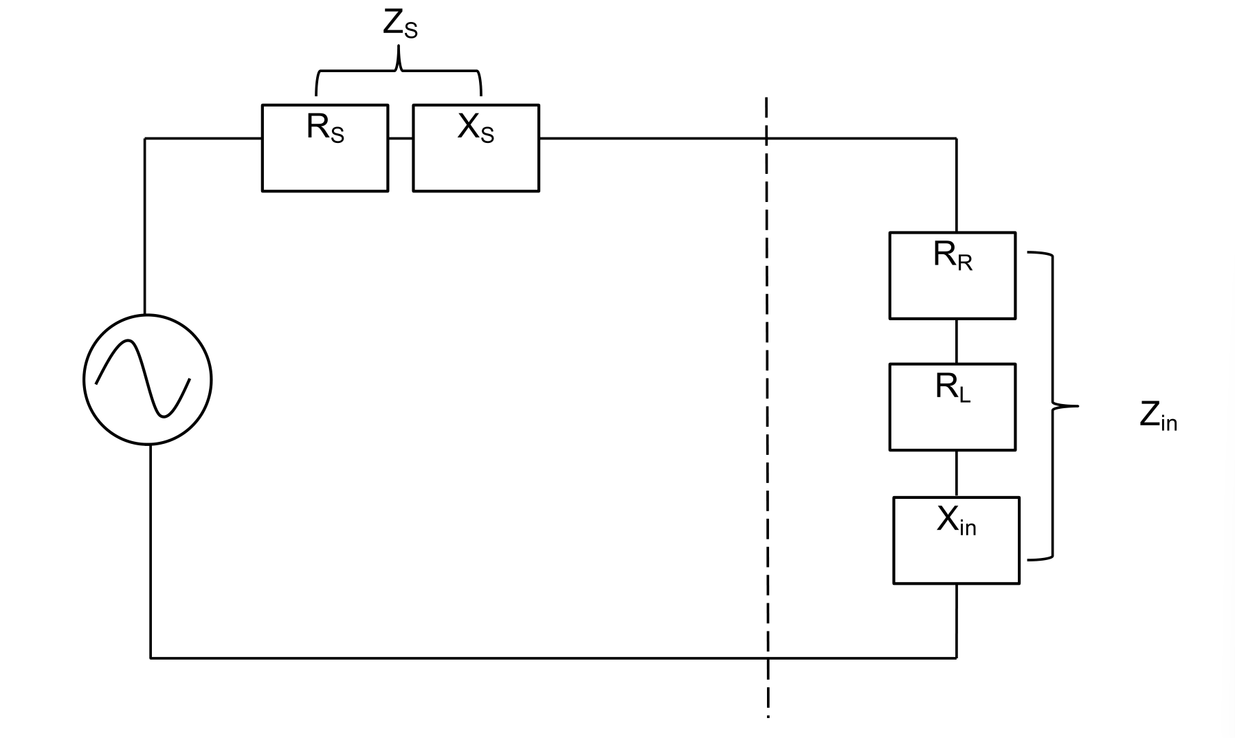
Impedance matching can be visualized using the equivalent circuit of the transmitting antenna. Maximum power transfer can only be achieved when \(Z_S = Z_{in}\):

Voltage Standing Wave Ratio (VSWR)

If there is impedance mismatch, it may result in some energy being reflected back, leading to the generation of standing waves. We use the Voltage Standing Wave Ratio (VSWR), denoted as \(s\), to describe the characteristics of these standing waves. It is defined as the ratio of the maximum and minimum voltages (or calculated based on the ratio of currents) on the transmission line:

\[ s = \frac{V_{max}}{V_{min}} = \frac{I_{max}}{I_{min}} \]

Alternatively, the VSWR can also be calculated based on the amplitudes (or powers) of the incident voltage \(V_{forw}\) and reflected voltage \(V_{vref}\):

\[ s = \frac{|V_{forw}| + |V_{refl}|}{|V_{forw}| - |V_{refl}|} = \frac{\sqrt{P_{forw}} + \sqrt{P_{forw}}}{\sqrt{P_{forw}} - \sqrt{P_{forw}} \]

The ratio of the reflected voltage \(V_{vref}\) to the incident voltage \(V_{forw}\) amplitude is called the Reflection Coefficient \(r\):

\[ r = \frac{V_{refl}}{V_{forw}} \]

Hence, VSWR can also be calculated using the Reflection Coefficient:

\[ r = \frac{1 + |r|}{1 - |r|} \]

Additionally, we define the logarithmic form of the Reflection Coefficient as Return Loss \(a_r\):

\[ a_r = -20\log |r| \]

\[ = -20\log\frac{V_{refl}}{V_{forw}} = -10\log\frac{P_{refl}}{P_{forw}} \]

There are various parameters for measuring impedance matching quality, and their simple correspondence is as follows:

VSWR	R	\(a_r\)	Reflective Energy
1.002	0.001	60dB	\
1.01	0.005	46dB	\
1.1	0.05	26dB	0.2%
1.2	0.1	20dB	0.8%
1.5	0.2	14dB	4%
2.0	0.33	9.5dB	11.1%
2.0	0.5	6dB	25%
5.0	0.67	3.5dB	44.4%

Antenna Factor

The antenna factor (also known as antenna coefficient or antenna factor) is typically used for receiving antennas and is defined as the ratio of electric field strength to the output voltage measured at the feed point (under 50Ω):

\[ K=\frac{E}{V} \]

Most of the time, it is expressed in its logarithmic form (dBm):

\[ k=20log K \]

If the antenna has been factory calibrated, the value of the antenna factor is generally fixed. The relationship between the antenna factor and actual gain is given by:

\[ K=\frac{9.73}{\lambda \cdot \sqrt{G}} \]

\[ k=-29dB+20log(\frac{f}{MHz})-g \]

Bandwidth

The antenna's bandwidth parameter is used to measure its usable frequency range, within which the antenna's performance meets the requirements. The standard for bandwidth is usually impedance matching (VSWR < 1.5), although gain or sidelobe suppression, among other parameters, can also be used as bandwidth criteria.

For broadband antennas, the ratio of the highest to lowest usable frequencies is determined. For example, a 2:1 ratio is called a two-octave bandwidth, and a 10:1 ratio is called a ten-octave bandwidth:

\[ BW=\frac{f_H}{f_L} \]

Broadband antennas are defined as BW≥2. There is another definition of bandwidth that applies only to narrowband antennas:

\[ BW=\frac{f_H-f_L}{f_C}\cdot100\% \]

Here, \(f_C\) represents the center frequency. The value of this bandwidth can exceed 100% (up to 200%).

References and Acknowledgments

• "Antenna-Basics_Rohde&Schwarz"
• "如何選擇天線於微波系統_Rohde&Schwarz"
• Antenna Gain | WLAN Antenna Quick Start
• What Is Antenna Gain

Original: https://wiki-power.com/ This post is protected by CC BY-NC-SA 4.0 agreement, should be reproduced with attribution.

This post is translated using ChatGPT, please feedback if any omissions.